

Aggregate Production Plan for A Natural Rubber Production CompanyUche E. Uche
Department of Mechanical Engineering, Air Force Institute of Technology, Kaduna, Nigeria
*Correspondence to: Uche E. Uche
Citation: Uche UE (2024) Aggregate Production Plan for A Natural Rubber Production Company. Sci Academique 5(1): 29-49
Received: 24 January, 2024; Accepted: 12 March, 2024; Publication: 23 March, 2024
Abstract
The objective of the study is to put in place an aggregate rubber production plan to be considered during a planning horizon of a year or two ahead of the current year as requested by an investment company. In this study the resources are aggregated in tons of rubber produced. Data collection is carried out by three methods, namely direct observation, interviews, and from documentations, such as reports and internal company records. The cuplump production forecast is based on 12-year quarterly rubber production data set of six rubber clones on the company own plantation. The rubber tree yield parameters are estimated by maximum likelihood using Structural Time Series Analyser, Modeller and Predictor software (STAMP) to obtain the field production for the incoming year. The operation management (OM5) general solver on Excel spreadsheet for transportation method is deployed to produce the incoming year aggregate rubber production plan that optimizes the cost of rubber production. The result is a good mix of regular time rubber tappers, overtime tapping and subcontracting for each quarter, that meets the factory processing and market demand of 1830 tons of rubber at an optimal cost of N1, 563,730 for the planning horizon January- December. The study offers a robust guide for the establishment of an annual aggregate rubber production plan for natural rubber production.
Keywords: Aggregate; Planning; Transportation; Maximum Likelihood; Cuplump; Crumb
Introduction
The latex that flows from a rubber tree during tapping is a suspension of rubber globules (cis-1, 4-polyisoprene) in water. It consists of 35% rubber, 60% water, 5% resins, fatty acids, proteins and other substances [1]. The rubber can be recovered as a liquid, then coagulated at the processing plant by adding acid (formic or acetic acid) or can be harvested in the field as a solid following natural coagulation. Two processing methods are most frequently used for producing natural rubber from latex: processing in the form of sheets or in the form of crumb. The factory rubber processing flow chart is as depicted in figure 1. The cup lumps brought from the field and local purchases are stored for maturity, soaked in water for some time to soften and precleaned, then fed into size reducing machines – pre-breaker, slab cutter, hammer mill 1 and 2 to be first broken up into small bits or crumbs before passing through four sets of creeping machines. The crepes are then put into the shredder or extruder then through fine creepers and shredder before being washed in the bank pool and placed in dryer boxes for dripping. And then into the drying chamber to be dried by hot air at 125oC/120oC wet and dry ends respectively by a diesel-fired dryer. The dry crumbs are cooled for 8 minutes, discharged, weighed, and pressed into lots of 33.33kg size to form bales. They are technically graded and wrapped in a 0.004mm transparent polythene sheet as figure 4. Thirty-six bales are packed in a pallet amounting to 1.2 tonnes. After processing, the boxes are removed from the dryers and the contents removed. Some pieces of the leftover get stocked in the boxes. The boxes are therefore soaked and cleaned in the washing station before re-use. Field coagula are only suitable to produce TSR10 and TSR20 grades, not TSR5 which comes from latex coagula because of the high dirty content.
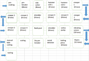
Figure 1: Flow chat for a rubber processing line.
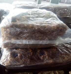
Figure 2: Crumb Rubber.
Natural rubber (NR) accounts for around a third of total rubber production compared to synthetic rubber produced from petrochemicals. It has specific properties such as resistance to heating and micro splitting that makes it a difficult product to replace [2]. Southeast Asian nations of Thailand, Indonesia, and Malaysia account for 74% of World production and 90% of world exportable production. Nigeria contributes less than 2% of world natural rubber of African’s 5% share. The percentage consumption of natural rubber in the world is as shown in Figure 3. Asia accounts for 53% of world natural rubber consumption.
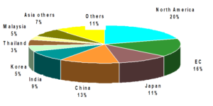
Figure 3: Natural Rubber Users [3]
Each car tyre has about 15-20% NR representing about 30-40% of the tyre elastomers while truck tyre contains about 30-40% NR (75-90% NR/elastomers) amounting to 25 Kg NR per 75 Kg truck tyre [3].
Natural rubber plays an important role in the environment and economy of nations producing it. Natural rubber, could potentially replace synthetic materials and fossil fuels, therefore reducing greenhouse gas (GHG) emissions, and on the other hand can contribute to climate change mitigation by increasing carbon sinks. It can also support the adaptation of other systems to climate change [4]. Moreover, in this era of increasing cost of fossil fuel the unsaturated fatty acid in rubber seeds oil can decrease the oxidation stability of fuel if the rubber seed is used as feedstock for biodiesel [5]. The rubber seed is therefore a valuable non-edible oil source for biodiesel production [6]. In Nigeria, it provides employment for the inhabitants of the rubber belt. Again, it is a major raw material for some vital home industries. Further, it earns foreign exchange for Nigeria through the export of rubber. Once latex yield declines, the rubber tree can be used as a timber source, reducing the need for deforestation for timber. To sustain these roles, field rubber production processes must be competitive, predictive, and assured through robust forecast of the future yield performance of the rubber plantation for aggregate rubber planning required to improve the programming efficiency of the processing centres and allow the estates and factory to plan transport facilities for rubber crop in advance.
As the name aggregate implies, aggregate planning involves combining the relevant resources into general terms or an overall aggregate for planning purposes. In other word, it requires an overall measure of output of diverse activities such as demand, inventory, workforce, production, capacity etc. [7]. The objective of aggregate planning can therefore be conflicting because of the many functional areas in an organization that give input to aggregate plan. These include to minimize costs/maximize profits, minimize inventory investment, minimize changes in production rates, minimize changes in workforce levels, maximize customer service and maximize utilization of plant and equipment. Hence for aggregate output plans, each plant, facility, or division requires its own aggregate capacity plan so that capacity and demand must be in balance.
An aggregate production plan for an agricultural company which experiences seasonal shift in its production due to vagaries of weather is a statement of its field production rate, work-force levels and inventory holdings based on estimate of processing requirements and capacity limitations – time phased and projected into the future [8]. It is predicated on the existence of an aggregate unit of production, such as the average number of items, or in terms of weight, volume, production time, or monetary value [9]. Aggregate planning is the essence of intermediate–range planning done within the limitation of long-range plan [10].
Two strategies are available to achieve the aggregate plan objectives. On one hand is the active aggregate planning strategy whose objective is to smooth out the peaks and valleys of demand during the planning horizon to obtain a smoother load on the production facilities. These include use of complementary products and creative pricing. On the other hand, passive strategies aim to absorb the fluctuation in demand through work force size, work rate, inventory, subcontracting and capacity utilization [11]. In other words, in the Exact Production Plan, the variable is the number of workers, while the demand remains constant. According to [10], the constraint of this plan is that the production must be equal to the demand. The model for this type of plan is shown in equation 1:
𝑈𝑛𝑖𝑡𝑠 𝑝𝑟𝑜𝑑𝑢𝑐𝑒𝑑 per 𝑤𝑜𝑟𝑘𝑒𝑟 = 𝑈𝑛𝑖𝑡𝑠 𝑝𝑟𝑜𝑑𝑢𝑐𝑒𝑑 per 𝑦𝑒𝑎𝑟/ 𝐷𝑎𝑦𝑠 𝑤𝑜𝑟𝑘𝑒𝑑 per 𝑦𝑒𝑎𝑟 (1).
For the Constant Workforce Plan the variable is the production rate while the number of workers each month is a constant. The formula for the development of this plan is presented in equation 2:
𝑊𝑜𝑟𝑘𝑒𝑟𝑠 𝑛𝑒𝑒𝑑𝑒𝑑 = 𝑑𝑒𝑚𝑎𝑛𝑑 per 𝑚𝑜𝑛𝑡ℎ/ (𝑑𝑎𝑦𝑠 per 𝑚𝑜𝑛𝑡ℎ × 𝑢𝑛𝑖𝑡𝑠 per 𝑤𝑜𝑟𝑘𝑒𝑟 per 𝑑𝑎𝑦) (2)
Methods for aggregate planning include graphical method, transportation model, linear and goal programming. Graphic strategy does not guarantee optimal production plan [12]. Application of the transportation method is also limited because it does not account for cost of production level changes [13].
In this study an investment company was considering an investment in a rubber processing company located in Abia State Nigeria. The company is an indigenous company involved in rubber plantation management that includes exploitation and processing of natural rubber to crumb rubber. It produces technical standard rubber TSR 10 and TSR 20 brands of crumb rubber essentially for export. While the demand for crumb rubber fluctuates from season to season to peak in the third quarter the more challenging and limiting factor for crumb rubber production is the supply of rubber cuplump which is the material processed into crumb rubber for export. The company installed crumb rubber processing capacity is 8 tons dry rubber per day (1870 tons/year), which represents the minimum demand on the field for rubber production. This line can reliably be fed from the 1250 hectares’ rubber plantation owned by the company with an estimated production of 2080 tons per annum (1664.4kg/ha) at full maturity. A due diligence requests is made by the investment company to determine the best production plan that shows how the organization will work toward longer term objectives in the face of volatile demand of the factory product and limited capacity for cuplump supply from own rubber plantation and environ. The objective being to put in place an aggregate rubber production plan to be considered during a planning horizon of a year or two ahead of the current year.
Methodology
The study is within the framework of the terms of reference (TOR) of the due diligence request by an investment company. Information on operation status is collected by survey techniques (field research) aims at eliciting and proffering solution to problems in the rubber industry understudy. Data collection is carried out by three methods, namely direct observation, interviews, and from documentations, such as reports and internal company records. Hence, evaluation research method is adopted. The cuplump production forecasting is based on 12-year quarterly rubber production data set of six rubber clones – GT1, PB217, PB260, PB28/59, PB324 and RRIM703. Regular recording of girth is a valuable index of tree growth rate and means to predict opening date. It commences as early as a year after planting and repeated at 6 monthly intervals up to the time of the last opening which generally takes place about a year after the first opening. Tree girth is measured at 100cm above the bud union on individual tree before opening. Once a plot of trees is of the right girth (50cm at 1m) and tapping density (40%) the plot is opened for tapping. The trunk circumference is thereafter measured using a measuring tape at 1.7 metre height – previously marked with white paint. The plantation has been opened since 1998 and tapped on S2D4 6d/7 tapping intensity. In other words, the taping system used is the half spiral cut (S2) from tapping year one to nine and alternate quarter cut (S4) and half spiral cut thereon at fourth daily frequency (D4), six days tapping followed by one day rest(6D/7). Hence trees are tapped 6 times per month. The production is collected, weighed and recorded in replicates. It is then analyzed and expressed in gram per tree (g/t) and in kilogram per hectare (kg/ha) by replicates for analysis of variance. Ethrel 10% is routinely used to enhance production – 1 gram of stimulant is applied on 1 cm band of the tapping panel after dilution with water to 2.5, 3.3 or 5% concentrations depending on the clone. The stimulation frequencies are variable depending on the clone and tapping year. A fairly standard and consistent tapping policy was followed over the period under study in the supplementary information. The study is to estimate the rubber yield parameters to be used to forecast the incoming year rubber production per tree and to establish an aggregate rubber production plan for the investment company.
State space specification of structural time series model was considered as a framework to implement the rubber tree production model that incorporates five main rubber production decision variables, namely, tree girth, tapping system, tapping height, stimulation level and stimulation round. The girth at which tapping begins is a key element affecting the economy of a rubber plantation [14]. If tapping is started when the trees are too young and slender subsequent growth and girthing will be poor rendering the tree highly susceptible to wind damage [15] To have a higher number of latex vessels, girth increment is a very important factor. Rubber tree yield response to stimulation (ethrel) depends on a number of factors including age and the clone. Other factors include nutrient status and tapping history, concentration yield stimulant and rounds of application. Hence the major factors contributing to response to stimulation that can be manipulated are the type of active ingredient, its concentration, the method of formulation, the mode of application, the frequency of application and the taping system adopted [15]. Finally, there is generally higher response to stimulation at higher and shorter cut, possibly due to higher magnesium content of latex at higher levels in the tree which causes early plugging. This is supported by the work of [16], in which the opening of PB 235 rubber clone at 1.20 m above the ground level gave approximately 7% more rubber than the opening at 0.75 m above the ground level. All the rubber yields co-variable form the explanatory variables in forecasting rubber tree yields a year ahead. The beginning of the study is defined as the year when the plantation came into production (1998) while the end of the study is the time when the study is realized.
Kalman filter was used to minimize the prediction error variance by data assimilation. The rubber yield aggregation is realized at the level of plantation yield prediction for the planning horizon. The production from regular workforce, overtime, outsourcing, and inventory were aggregated in tons of rubber produced using the computer software OM5 general solver Tableau solution of transportation method on Excel spreadsheet.
In the study model a series of 48 observed rubber yield values per clone are decomposed into unobserved trend, seasonal and noise components to facilitate the description of the series in terms of its component of interest such as the seasonal behaviour of yield and the trend movement. The yield per tree (Y gm/tree) is modelled as stochastic level with stochastic seasonal plus irregular, AR (1) and five explanatory variables (tapping cut height, tapping system (1/2 or 1/4 spiral cut), ethrel stimulation levels and frequency per physiological year) as depicted in equation (3).
Y = Trend + Seasonal + Irregular + AR (1) + Explanatory variables (3)
where Y = rubber production per tree.
The parameters are estimated by maximum likelihood using Structural Time Series Analyser, Modeller and Predictor software – STAMP [16]. The model is adopted to minimize the noise associated with a time dependant product such as the yield of rubber tree and weight of wet cuplump [18].
The prediction of one-step-ahead yield per tree is within the framework of Gauss-Markov- Discrete-Time Kalman filter model [19]. The software estimates the yield per tree for the incoming year. The predicted yield per tree is used to determine the number of rubber trees required to meet rubber production demand by the factory and the tapping workforce level using the agreed tapping task size. The information is subsequently used to establish the annual tapping aggregate rubber production plan that meets the company rubber processing and market demand.
Transportation method is employed for the aggregate rubber production planning because it is particularly helpful in determining anticipation inventory since the objective is to minimize rubber tree exploitation cost and maximize the use of installed rubber processing facility. Secondly, the rubber tapping work force, levelled for each period are input rather than output in the rubber production plan. A level strategy is employed with overtime rather than chase strategy because rubber tapping has steep learning curve compounded by the dearth of rubber tapping workforce in the Nigerian labour market. The transportation method proposed in the study is based on the assumptions that the factory rubber demand forecast is available for each quarter, along with capacity limits on tapping overtime and outsourcing of lump supply. Finally, and more important, quantity of rubber produced is linearly related to the cost of production, a prerequisite for the application of transportation method to aggregate planning. The production from regular tappers, overtime, outsourcing, and inventory were aggregated in tons of rubber produced. The operation management computer software OM5 general solver on Excel spreadsheet for transportation method is deployed to produce the incoming year aggregate rubber production that optimizes the cost of rubber production.
Hence the aggregate rubber production planning strategy is the level passive strategy that meets fluctuation in regular cuplump production with overtime, subcontracting and inventory. Constant number of tapers is kept at a level to satisfy demand during the planning horizon. The number of tapers recruited at the beginning of the planning horizon is such that undertime is minimal while overtime and outsourcing of cuplump is maximized in the peak period of July to December. A spare taper is also available for relieve duty for the team. The unit leader divides the plantation into four tapping parts for the four-day tapping frequency system (D4) under the direction of the plantation manager.
The aggregate production planning steps begin from forecasting the field production, having established the demand (processing capacity) and continue with the aggregate planning of cuplump production. Of the two types of aggregate planning which are usually determined by means of mathematical models: Exact Production Plan; (vary workforce) and Constant Workforce (vary inventory and stockout), the fixed workforce strategy is adopted as follows:
Assumption: Hiring and firing of tapers are disallowed. Rubber cuplump supply rates can fluctuate only by using overtime and outsourcing.
Data:
cit = unit production cost for rubber clone i in period t (exclusive of labor costs)
hit =inventory carrying cost per unit of rubber clone i held in stock from period t to t+ 1).
rt = cost per man-day of regular taper in period t
ot = cost per man-day of overtime taper in period t
dit = forecast demand for rubber clone i in period t
mi = man-day required to produce one unit of rubber clone i
ℜt= total man-day of regular taper available in period t
Ōt= total man-day of overtime tapers available in period t
Ii0 = initial inventory level for rubber clone i
T = time horizon in periods
N = total number of rubber clones
Decision Variables:
Xit = units of rubber lump i to be produced in period t
Iit = units of rubber lump i to be left over as an inventory in period t
Rt = man-day of regular taper used during period t
Ot = man-day of overtime taper used during period t
i = Rubber clone: GT1, PB217, PB260, PB28/59, PB324 & RRIM703.
The linear program for this model is to:
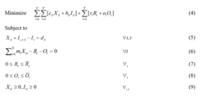
Results and Discussion
Estimation of the Plantation Cup Lump Production Capacity
The analysis presented herein applies to the 12-year quarterly rubber production data (Table 1 & Supplementary file), of six rubber clones – GT1, PB217, PB260, PB28/59, PB324 and RRIM703 that predominant the company own plantation. Tht, gth, st are the tapping height, tree girth and stimulation respectively. The rubber clones were used for the determination of yield response to girth increment, tapping height, tapping system, concentration and rounds of stimulation. The yield data used consist of daily data averaged per tree in gram and summed per month/quarter. The 12-year quarterly dry rubber production per tree for each rubber clone and the co-variables of rubber tree production provided adequate data for the rubber yield parameter estimation and for forecasting the seasonal breakdown of the coming year rubber production using Kalman filter. The one-year-ahead estimates were used to prepare the aggregate rubber production plan for the plantation.
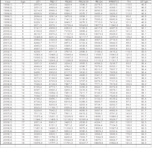
Table 1: 12-Year Yield Data of Six Company Rubber Clones (g/tree/year).
Preliminary analysis
This includes data characterization and plot inspection.
Data characterization
Data characterization is carried out to ascertain the integrity of collected data and to adopt appropriate statistical tool for the analysis. The density distribution shown in Figure 4 is estimated as a smoothed function of the histogram by STAMP using a normal or Gaussian kernel to give the estimated cumulative distribution function of the rubber production data.
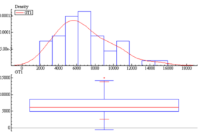
Figure 4: Density Distribution and Box Plot of GT1 rubber yield data.
The Box plot of Figure 4 shows that the smallest value is 2605g and the largest is 15078g for the GT1 rubber clone. Data characterization of all the clones using Box plot is given in Table 2. In the table two clones, GT1 and PB217 have outliers due to change in stimulation from 2.5 to 5% for 2009 physiological year.
| Clones | Minimum | Maximum | 1st QL | Median | 3rd QU | IQR | LW | UW | Outlier |
| GT1 | 2605 | 15078 | 4882 | 6230 | 8623 | 3741 | -730 | 14235 | 15078 |
| PB217 | 3081 | 17777 | 5828 | 7406 | 10083 | 4255 | -555 | 16466 | 17777 |
| PB260 | 3229 | 13587 | 5031 | 6980 | 99467 | 4436 | -1623 | 16121 | – |
| PB28/59 | 2658 | 12118 | 4736 | 6402 | 9133 | 4397 | -1860 | 15729 | – |
| PB324 | 2279 | 16610 | 5377 | 7715 | 9902 | 4525 | -1411 | 16690 | – |
| RRIM703 | 2574 | 12370 | 5014 | 6620 | 8722 | 3708 | -548 | 14284 | – |
| *QL = Lower quartile, QU = Upper quartile, IQR = Interquartile range, LW = Lower whisker, UW = Upper whisker. | |||||||||
Table 2: Result of Box plot data characterization (gm/tree/year).
Plot inspection
Figure 3 shows the actual plot of GT1 rubber clone yield per tree from January 1998 to December 2009. The graph shows a seasonal pattern of yield usually associated with tropical climate of dual seasons-dry and wet season within a year. The overall trend of the series is constant over the years. Its salient characteristics are a trend, which represents the long-run movements in the series, a seasonal pattern which repeats itself more or less every year and the irregular components which reflects non-systematic movement in the series.
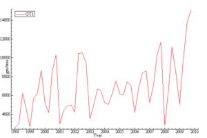
Figure 5: GT1 g/tree quarterly actual series plot.
STAMP output (Figure 5) suggests that cyclical event is absent. Hence a model of the series needs to capture these characteristics. The choice of model is therefore informed by the decomposition of the series into its components as shown in Figure 6. The model to be considered initially is therefore the basic structural time series model (BSM) without cycle [17] which is given by:
![]()
where µt is the local level component modelled as the random walk , µt+1 = µt +ξt,
yt is the trigonometric seasonal components and εt is a disturbance term with mean zero and variance σ2ε. As displayed in Figure 6, the seasonal effect hardly changes and is therefore considered fixed. The estimated level does pick up the underlying movement of the series and the estimated irregular is alright.
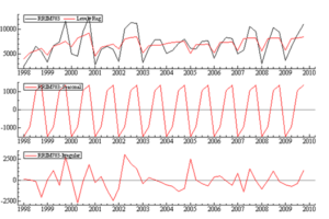
Figure 6: RRIM703 g/tree stochastic model decomposition.
Incoming year rubber production forecast
The rubber production models obtained for the various rubber clones are expressed in state-space form as shown in equation 11 for GT1 rubber clone:
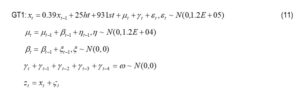
where xt is the yield estimate of the clone at the start of period t, zt is the current yield, µ is the: yield trend at t=1, β is the rate, is the seasonal effect, ω, ξt ,ϒt , ε are the error terms and ht, gt, st are the tapping height, tree girth and stimulation respectively. The state space equations for other rubber clones were similarly developed.
Incoming year rubber production estimated level is displayed in Figure 7 for PB 217 rubber clone; the filtered estimator is based on only the past data, that is E(µt|Yt-1) where µt is yield estimate given the immediate past measurement Yt-1 and the smoothed estimator is based on all the data, that is E(µt|Yn). The filtered estimator lags the shocks in the series as is to be expected since this estimator does not take account of current and future observations. Further, the initial distribution of the filter is estimated by maximum likelihood from 1998 to 2000 observations. The graph further shows that the model makes yield forecasts adequately for PB217 rubber clone. The smooth rise in production clearly depicts the industrial character of PB217 rubber clone. It is consistent with prior knowledge- content validity.
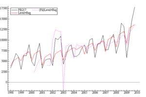 Figure 7: Data (solid black) with filtered (dotted) and smoothed (solid red) estimators.
Figure 8 shows the forecast of rubber production per tree for the incoming year (2010/11) for GT1 (tabulated in Table 3). It reflects the trend and seasonal movements captured by the structural time series model. The lines on the either side of the forecast function are based on the estimated root mean square error (RMSE) and indicate the prediction interval that limits the rubber production estimate to be used for the aggregate rubber production plan. As the forecast horizon increases so does the uncertainty attach to the forecasts and the prediction interval becomes wider.
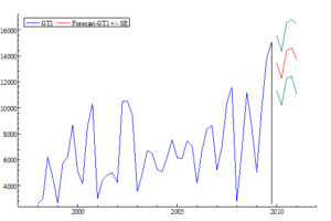 Figure 8: Incoming year rubber clone yield forecast (gm/tree).
| Quarter | Forecast | Std Error | Left Bound | Right Bound |
| 1 | 13437 | 2119 | 11317 | 15556 |
| 2 | 12300 | 2078 | 10221 | 14379 |
| 3 | 14415 | 2147 | 12268 | 16563 |
| 4 | 14624 | 2179 | 12445 | 16803 |
Table 3: Yield Forecasts (g/tree/year) at 68% confidence interval from period 2009(4) forwards for GT1.
Table 4 depicts the 2010/11 physiological year actual rubber production per tree to model forecast for all six rubber clones. The first quarter is excluded because of change in rubber tree exploitation practice that affected the actual yield. In carrying out the significance test of actual to forecast yield, the rule is that if the modulus of the variate-value d, is greater than 1.96, the null hypothesis that actual yield observed come from the model forecast is rejected at 5% (0.05 probability) significant level and if otherwise i.e., d<1.96 it is accepted. Similarly, for |d| > 2.58 at 1% (0.01 probability) significant level and |d|> 3.29 at 0.1% (0.001probability) significant level the null hypothesis is rejected and otherwise accepted. The variate-value d is given by equation 12.
![]()
where, x = the actual rubber yield per tree
µ = model forecast rubber yield per tree
σ = standard error of the forecast.
The numerical value of d is less than 1.96 and hence the null hypothesis that the actual yield is within the forecasted value is accepted at 5% significant level for the rubber clones and seasons studied. The upper and lower bounds of the rubber yield forecast as outputted by STAMP are also shown in Table 4 to further confirm the validity of the model.
| Actual | Forecasted | Standard error | Lower bound | Upper bound | Variate value(d) d=(x-µ)/σ
< 1.96 |
||
| Treat | Quarter | Total | |||||
| GT1 | 2 | 10857 | 12300 | 2079 | 10221 | 14379 | -0.694 |
| 3 | 13230 | 14415 | 2147 | 12268 | 16563 | -0.552 | |
| 4 | 13987 | 14624 | 2179 | 12445 | 16803 | -0.292 | |
| PB217 | 2 | 14220 | 13832 | 2070 | 11761 | 15902 | 0.187 |
| 3 | 15096 | 15499 | 2097 | 13401 | 17597 | -0.192 | |
| 4 | 15287 | 16518 | 2106 | 14412 | 18624 | -0.585 | |
| PB260 | 2 | 10847 | 9647 | 2736 | 6911 | 12383 | 0.438 |
| 3 | 13035 | 11695 | 2893 | 8802 | 14589 | 0.463 | |
| 4 | 11774 | 11771 | 2989 | 8782 | 14760 | 0.001 | |
| PB28/59 | 2 | 9224 | 9102 | 2169 | 6933 | 11271 | 0.056 |
| 3 | 11533 | 10832 | 2283 | 8549 | 13115 | 0.307 | |
| 4 | 9016 | 11505 | 2344 | 9161 | 13849 | -1.062 | |
| PB324 | 2 | 12159 | 13157 | 1859 | 11298 | 15016 | -0.537 |
| 3 | 13442 | 15059 | 1857 | 13202 | 16917 | -0.871 | |
| 4 | 13503 | 15079 | 1856 | 13223 | 16936 | -0.849 | |
| RRIM703 | 2 | 10257 | 7907 | 2116 | 5791 | 10023 | 1.111 |
| 3 | 13119 | 9941 | 2241 | 7700 | 12183 | 1.418 | |
| 4 | 11325 | 10329 | 2360 | 7970 | 12689 | 0.422 |
Table 4: Significant test of Actual Yield to Model Forecast (g/tree/year).
Aggregate Rubber Production Plan for the Plantation
The data collection in aggregate planning is production capacity and production costs. The company plantation production capacity consists of regular production capacity, overtime capacity, and the subcontracting policy by the company. In Table 5 is the estimated cup lump production capacity per quarter.
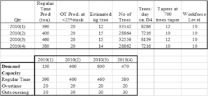
Table 5: Rubber production capacity estimation for 2010.
Production costs include regular production costs, production costs of overtime and subcontract, inventory costs, and inventory shortage costs as follows:
- Maximum allowable overtime is 25 percent of the tapping task size.
- Outsourcing is limited to 30 tons per quarter.
- No backorder or stockouts are permitted.
- The per unit holding cost for the beginning inventory in period 1 is 0 because it is a function of previous production planning decisions.
- No holding cost is charged on the target inventory at the end of the planning horizon because an ending inventory is specified; in this regards it is a sunk cost.
- Initial inventory: There is 40 tons of dry rubber available at no additional cost because it is used in period 1.
- Carrying cost is =N=100 per ton per period if units are retained until period 2, =N=200 per ton until period 3, and so on. If the units are unused during any of the four periods, the result is =N=300, plus =N=100 to carry it forward to the next planning horizon, for =N=400 total if unused.
- Regular time: Cost per kg is =N=830 if the rubber is used in the month produced; otherwise, a carrying cost of =N=100 per ton is added per ton retained.
- Overtime: Cost per unit is =N=910 per ton if the rubber is used in the month produced; otherwise, a carrying cost of =N=100 per ton is incurred as in the regular time situation. Unused overtime has zero cost.
- Subcontracting: Cost per ton dry rubber is =N=1000 plus any costs for units carried forward. There is no cost for unused capacity.
- Final inventory: A minimum inventory requirement of 40 tons must be available at the end of the planning horizon to provide for wet cup-lump maturation of two to four weeks and for the blending operation of rubber from the different rubber clones before processing.
The aggregate rubber production planning problem is summarized in Table 6.
| Beginning Inventory (ton) | 40 |
| Desired Ending Inventory (ton) | 40 |
| Holding Cost (=N=) | 100 |
| Regular Time (=N=) | 830 |
| Overtime (=N) | 910 |
| Subcontract (=N=) | 1,000.00 |
| Backorder Cost (=N=) | *9,999.00 |
| (* Use a very high value in this cell to disallow backorders). | |
Table 6: Summary of aggregate rubber production problem (per Ton).
Table 7 is a tableau of the work force levels, capacity limits, and factory rubber demand, beginning inventory level, and cost for each period of the planning horizon. The forecasted yield (Table 4&5) for the aggregate rubber production planning is the mean production per tree for the six rubber clones by quarter. The rubber yield aggregation is realized at the level of yield prediction for the planning process.
| Alternatives | Quarter | Unused | Total | ||||
| 1 | 2 | 3 | 4 | Capacity | Capacity | ||
| Beginning | 0 | 100 | 200 | 300 | |||
| Inventory | 40 | 0 | 40 | ||||
| 1 | Regular | 830 | 930 | 1,030 | 1,130 | ||
| Time | 90 | 220 | – | 80 | – | 390 | |
| Overtime | 910 | 1,010 | 1,110 | 1,210 | |||
| – | – | 20 | – | – | 20 | ||
| Subcontract | 1,000 | 1,100 | 1,200 | 1,300 | |||
| – | – | – | – | 30 | 30 | ||
| 2 | Regular | 9,999 | 830 | 930 | 1,030 | ||
| Time | – | 180 | 220 | – | – | 400 | |
| Overtime | 9,999 | 910 | 1,010 | 1,110 | |||
| – | – | 20 | – | – | 20 | ||
| Subcontract | 9,999 | 1,000 | 1,100 | 1,200 | |||
| – | – | 30 | – | – | 30 | ||
| 3 | Regular | 9,999 | 9,999 | 830 | 930 | ||
| Time | – | – | 460 | – | – | 460 | |
| Overtime | 9,999 | 9,999 | 910 | 1,010 | |||
| – | – | 20 | – | – | 20 | ||
| Subcontract | 9,999 | 9,999 | 1,000 | 1,100 | |||
| – | – | 30 | – | – | 30 | ||
| 4 | Regular | 9,999 | 9,999 | 9,999 | 830 | ||
| Time | – | – | – | 380 | – | 380 | |
| Overtime | 9,999 | 9,999 | 9,999 | 910 | |||
| – | – | – | 20 | – | 20 | ||
| Subcontract | 9,999 | 9,999 | 9,999 | 1,000 | |||
| – | – | – | 30 | – | 30 | ||
| Requirements | 130 | 400 | 800 | 470 | 30 | 1870 | |
Table 7: Tableau solution for 2010/11 aggregate rubber production plan (units as per Table 6).
The objective is to optimize rubber production and maximize the use of installed rubber processing facility. Thus, in period 1, the rubber exploitation manager will schedule 390 tons to be produced on regular time, 20 tons on overtime and 30 tons to be outsourced to local farmers. This provides 2nd quarter take-off stock of 350 tons. In period 2, 180 tons is produced in regular time to complement the 350 tons carried forward from period 1 for that quarters demand. Additional 220 tons is produced by regular time, 20 tons on overtime and 30kg outsourced to provide initial stock of 400 tons for the 3rd quarter need. Hence 460 tons is schedule on regular time to augment the 3rd quarter initial stock. Similarly, 20 tons on overtime and 30 tons subcontracted of 3rd quarter production provide for 4th quarter take-off stock. This is complemented by 380 tons, in regular time, 20 ton on overtime and 30 tons on subcontract for 4th quarter. Closing inventory (over capacity) for the planning horizon is 70 tons, allowing for usual shrinkage of unprocessed rubber in stock and blending for the next planning horizon (Table 8). Anticipatory inventory is the amount at the end of each quarter, where beginning inventory + Total production – Demand = End inventory. The production from regular workforce, overtime, outsourcing, and inventory were aggregated in tons of rubber produced using the computer software OM5 general solver Tableau solution of transportation method on Excel spreadsheet as shown in Table 7.
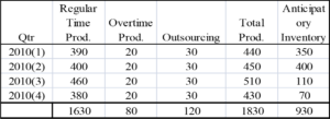
Table 8: Aggregate rubber production plan (ton).
The total cost of this prospective rubber production plan equals the sum of the products calculated by multiplying the allocation in each cell of the Tableau by the cost per unit in that cell. Computing the cost column by column yield a total cost of =N=1,563,730 for the 1870 tons of rubber. Hence the optimal solution produced an optimal cost of N1, 563,730 as shown in the OM5 printout -Table 9.
| Results | ||||
| Solver – Transportation Method for Aggregate Planning (=N=) | ||||
| Q1 | Q2 | Q3 | Q4 | |
| Costs | 391900 | 407200 | 401030 | 363600 |
| Total Cost | 15,63,730 | |||
Table 9: Optimal cost (OM5 printout).
Conclusion and Recommendation
An aggregate plan is a statement of production rate, work-force levels and inventory holdings of an industry based on estimate of processing requirements and capacity limitations. It therefore involves combining the relevant resources into general terms or an overall aggregate. In this study therefore, the aggregate plan for field crop production for the processing factory understudy is based on the one-year-ahead rubber yield prediction to obtain an anticipation stock of 70 tons for the year against the minimum target of 40 tons. This result is satisfactory being in line with the rubber processing policy that provides for natural shrinkage of wet rubber, cup lump maturation period and the blending of rubber from different rubber clones before processing. The plan also ensured that undertime of the tapping workforce is minimal while meeting the peak time demand of rubber. The result of the aggregate rubber production planning gave an optimal cost of N1, 563,730 for the planning horizon January- December. The transportation method implemented on OM5 Excel solver produced a good mix of regular time rubber taping, overtime taping and subcontracting for cuplump supply to meet the factory processing and /market demand of 1830 tons of rubber. The study offers a robust guide for the establishment of annual aggregate rubber production plan for an industry subject to the volatility of demand and raw material supply environment.
Conflict of Interest Declarations: The author hereby declares that there is no conflict of interest.
Reference
- Chin PS (1974) “Alternative Crumbling Agent for Hevea crumb Manufacture” Proceedings of the Rubber Research Institute of Malaysia Planters Conference. Kuala Lumpur: 219.
- Demange CA (1995) Hevea Strategies de selection, CIRAD – CP BP 5035,34032 Montpelliers Cedex 1, France.
- Uche EU (2004) Enhancing the International Competitive Edge of Rubber Processing in Nigeria” In: Report of the 3rd Nigerian Economic Summit Group Agricultural summit, pp 190-198
- Pinizzottoa S, Kadirb AASA, Gitzc V, Beuved JS, Naire L, et al. (2021) Natural Rubber and Climate Change: A Policy Paper. BRIEF 6.
- Sugebo B, Demrew Z, Biazen M (2021) Evaluation and Characterization of Rubber Seed Oil for Biodiesel Production in Biomass Conversion and Biorefinery. Springer Link.
- Sugebo B, Yebeyen D, Adugna A (2022) Latex yield variation among Hevea brasiliensis clones grown under the agroclimatic of South-West Ethiopia. Trees, Forests and People.
- Adam EE, Ebert RJ (2000) Production and Operations Management, Prentice-Hall of India, New Delhi.
- Krajewski LJ, Ritzman LP (1999) Operations management, Strategy and Analysis, Addisn-Wesley Publishing Company, Inc.
- Gallego G (2011) “Production Management” IEOR 4000, Lecture 5 p 173.
- Rizkya R, Sari M, Syahputri K, Siregar I (2021) The methodology of aggregate planning on lamp production based on transportation model. IOP Conference Series: Materials Science and Engineering.
- Cook TM, Russell RA (1984) Contemporary Operations Management, Prentice-Hall, Inc. New Jersey.
- Heizer J, Render B (2004) Principles of Operations Management Pearson Education International (U.S.A).
- Krajewski LJ, Malhotra MK (2022) Operations Management: Processes and Supply Chains, 13th edition, ISBN 978-0-136-86093-8, published by Pearson Education.
- Grist PG, Menz KM, Thomas (1995) “A modified version of the BEAM rubber agro- forestry model: small holders in Indonesia”, Canberra, CREA, ANU, Imperata Project Paper 1995/3.
- Webster CR, Lorimer CG (2005) Minimum opening sizes for canopy recruitment of mid-tolerant tree species: a retrospective approach. Ecological Applications 15: 1245-1262.
- Obouayeba S, et al. (2009). “Effect of tapping systems and height of tapping opening on clone PB235 agronomic parameters and its susceptibility to tapping panel dryness in south-east Cote d’Ivoire”. Journal of Applied Biosciences 24: 1535-1542.
- Koopman SJ, et al. (2009) STAMP: Structural Time Series Analyser, Modeller and Predictor. Timberlake Consultants, USA.
- Harvey A (2004) State Space and Unobserved Component Models: Theory and Application, Cambridge University Press.
- Igboanugo AC, Uche EU (2013) Minimum Variance Estimation of Yield Parameters of Rubber Tree with Kalman Filter. Nigerian Journal of Technology (NIJOTECH) 32: 81-92.